ARNy Plotter Documentation
This page provides documentation for the various plot
generation options available in the Plot RNA web
application. Each plot type is described along with its
purpose and usage, and technology stack used for.
The results are kept for 1 month for the moment, if you want a sooner deletion, you can send me a mail at louis.meuret at etu.u-paris.fr, I plan to add a settings on how much time results are kept.
Trajectories are processed as follows.
First, they are uploaded to the server in chunks, and an initial integrity check is performed to verify that both the topology and trajectory files can be opened. They are then loaded in MDAnalysis: if stride settings are specified, they are applied; if the trajectory or topology are not supported by one of the required tools, they are converted to XTC/PDB format.
The program then examines the selected plots and derives from them the set of calculations needed to satisfy all the requested plots. These calculations run in several steps: first, the basic calculations: RMSD, eRMSD, alongside any computations required for a single plot only; then, calculations that depend on the results of the first step. Finally, once all data has been produced, the plots are generated.
Everything runs asynchronously via Celery, which significantly reduces wait times. Once the calculations are complete, all results are sent to the server in Plotly JSON format for display.
The trajectory is either served from cache if available, or streamed from the server to the client for display in Mol* which is why loading in Mol* can sometimes take a moment.
How to Start
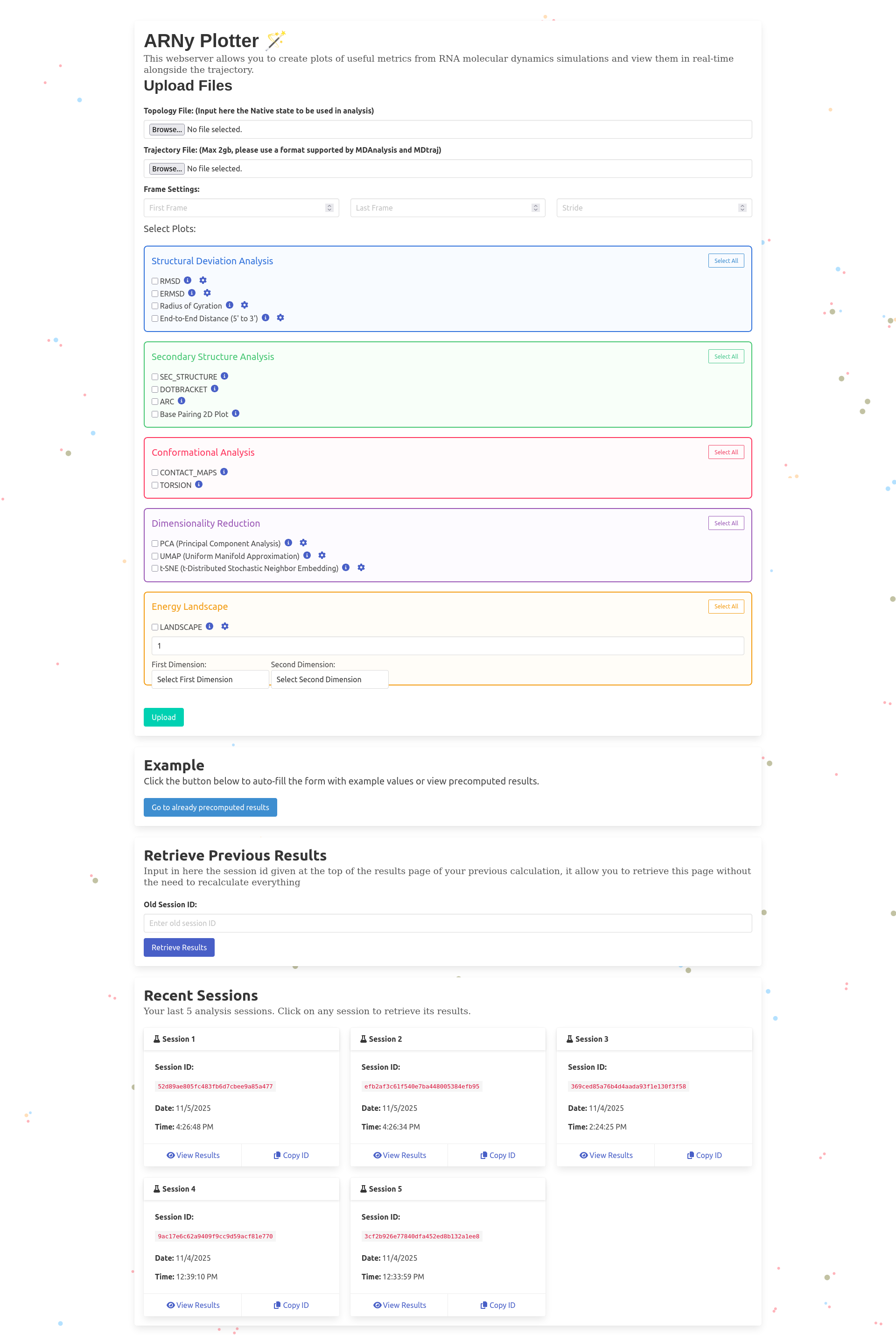
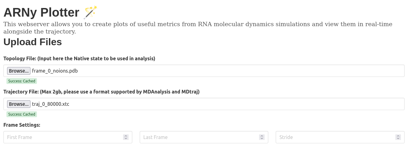
- A topology file, that couple as a native structure file and is used in all related calculations
- A trajectory file (multiple formats supported, primarily tested using XTC, but TRR, DCD are shown to work) if the file is not supported, an attempt is done to convert it to xtc format using MDAnalysis. It's possible to select specific atoms in the trajectory, in this case, the topology and the trajectory will both be filtered using MDAnalysis. For the moment, the upload limit on the main server is set to 500mb, this limit is not set when the server is self hosted.
- Set frame stride to skip frames
- Specify start/end frames to trim trajectory
- Leave empty to use full trajectory
- Note that the modifications are done on the server, the whole trajectory will still need to be uploaded
Choose which plots you want to generate from the available options described below, all the plots are described in the suite of this page
Click the "Upload" button to begin processing your data, at this moment, the website is going to send the form to the server: it can take some time, depending of the upload speed, the number of users, and the plots selected. No need to stay on the page while the computations are running: once the trajectory is sent to the server, you can leave and come back later to check the results using the session ID
Additional Options
- Click "Go to already computed results" to view an example, note that it's not going to recompute the data, hence the faster loading time.
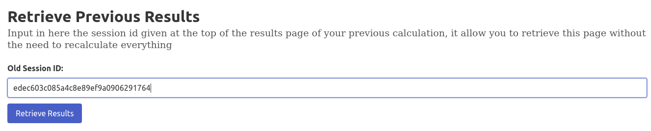
- Enter a previous session ID in "Retrieve Previous Results" to access past calculations
- If you have already sent calculations to the server, they are saved locally in a cookie, it allow us to add a pane showing the 6 last trajectories you've sent to the server, without the need to recompute the results.
The Analysis Page
Where everything you always wanted is..
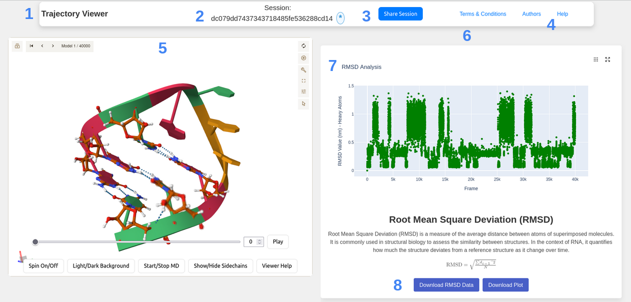
- Where all the controls about the webserver itself are, not related to the content
- The session ID is the unique identifier of the trajectory data you have sent, it's also the only way for the moment to get back the data you've computed
- If you want to share your exciting results with someone else, just click on this button: a link is created, and it will allow the others persons to access your data without the need to recompute everything.
- If you are lost, need some informations, click on Help !, the link redirect to this page where you can, hopefully, find all you need.
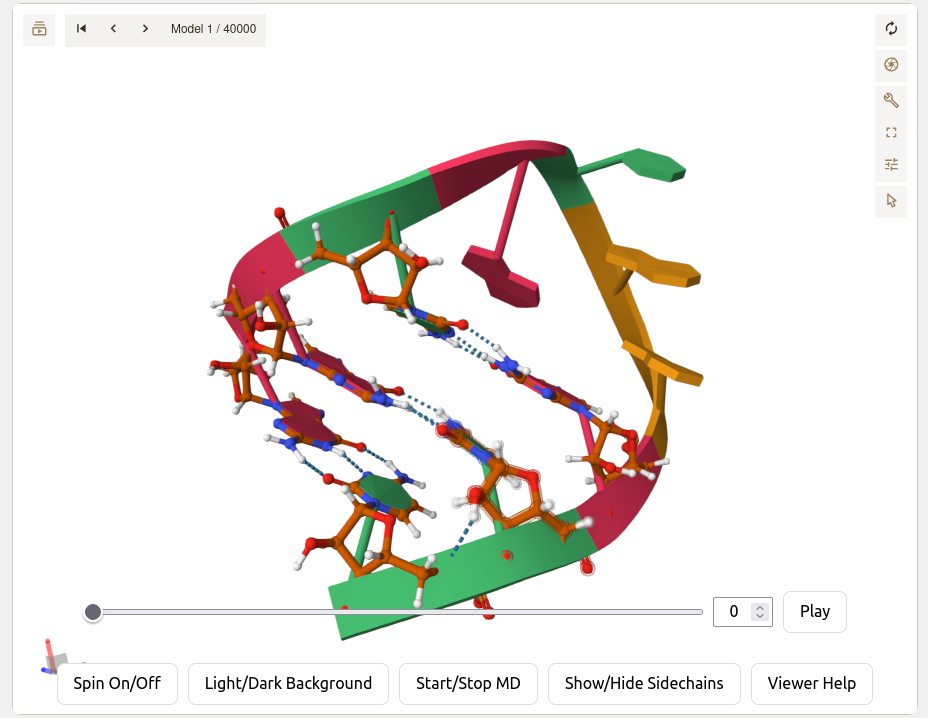
- In this Box, you can interact with the trajectory: change the displayed frame using the slider, the input box, or by clicking play. By toggling one of the 4 button under the slider, you can Spin the molecule, change the color of the background, display the sidechains Note that they are a lot of modifications that you also can do in the molstar viewer, where you can screenshot, change the frame, change what is displayed.
- Here is a scrollable plane where you can navigate between the differents plots you've created, each one has it's own box, composed by the plot first, then a title, a description, a formula if available and the possibility to download the data generated by the server.
- All the plot are currently generated using Plotly, if it's possible, some makers Highlight the current frame. Too much data and they cause the website to crash, by eating all your ram: if it's the case, try to add a stride, or select sections of your trajectories.
- When it's possible, buttons to download the data are appearing: you can click them to download in one case the data behind the plot, in general in csv format, or the plot itself, in html format usually.
1. Contact Maps Plot
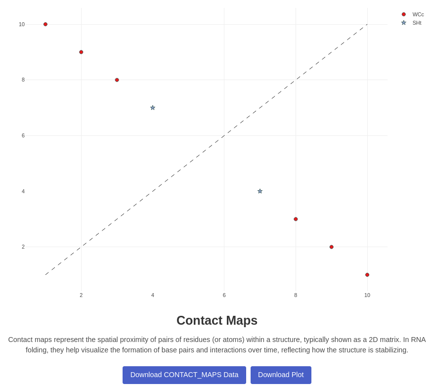
Generates a contact map plot for a given trajectory and native PDB file. Visualizes the contacts between residues in the RNA structure over the trajectory. Each cell correspond to index of atoms in the topology file, after parsing of MDAnalysis Visualisation is made using Plotly, different pairing are computed using Barnaba Annotation, and displayed at the right position When you change the displayed frame by the viewer, a call is sent to the server that will recompute the contact map, and update the current view, it takes between few hundred milliseconds for simple systems to multiple seconds for big systems Two buttons allow the user to switch between pairings and stackings mode: for the pairing mode the following contacts are highlighted:
| Code | Description | Color | Hex Code |
|---|---|---|---|
| Canonical Watson-Crick Pairs | |||
| WCc | Canonical Watson-Crick | #E41A1C | |
| WWc | Canonical Watson-Crick (alternative notation) | #E41A1C | |
| GUc | G-U wobble pairs | #FF7F00 | |
| Hoogsteen Pairs | |||
| WHc | Watson-Crick/Hoogsteen cis | #4DAF4A | |
| WHt | Watson-Crick/Hoogsteen trans | #984EA3 | |
| HWt | Hoogsteen/Watson-Crick trans | #984EA3 | |
| HWc | Hoogsteen/Watson-Crick cis | #4DAF4A | |
| HHc | Hoogsteen/Hoogsteen cis | #A65628 | |
| HHt | Hoogsteen/Hoogsteen trans | #F781BF | |
| Sugar Edge Pairs | |||
| WSc | Watson-Crick/Sugar edge cis | #377EB8 | |
| WSt | Watson-Crick/Sugar edge trans | #FFFF33 | |
| SWc | Sugar edge/Watson-Crick cis | #377EB8 | |
| SWt | Sugar edge/Watson-Crick trans | #FFFF33 | |
| SHc | Sugar edge/Hoogsteen cis | #66C2A5 | |
| SHt | Sugar edge/Hoogsteen trans | #8DA0CB | |
| HSc | Hoogsteen/Sugar edge cis | #66C2A5 | |
| HSt | Hoogsteen/Sugar edge trans | #8DA0CB | |
| SSc | Sugar edge/Sugar edge cis | #FC8D62 | |
| SSt | Sugar edge/Sugar edge trans | #BEBADA | |
| Other | |||
| XXX | Not classified or undefined | #C0C0C0 | |
For the stacking mode, the following stacking interactions are highlighted:
| Code | Description | Color | Hex Code |
|---|---|---|---|
| Directional Stacking Interactions | |||
| >> | Both nucleotides pointing right (parallel stacking) | #E41A1C | |
| << | Both nucleotides pointing left (parallel stacking) | #FF7F00 | |
| <> | Nucleotides pointing outward (antiparallel stacking) | #4DAF4A | |
| >< | Nucleotides pointing inward (antiparallel stacking) | #377EB8 | |
| Terminal Stacking Interactions | |||
| ss33 | 3'-3' terminal stacking (fallback classification) | #984EA3 | |
| ss35 | 3'-5' terminal stacking (fallback classification) | #FFFF33 | |
| ss53 | 5'-3' terminal stacking (fallback classification) | #A65628 | |
| ss55 | 5'-5' terminal stacking (fallback classification) | #F781BF | |
| Other | |||
| XXX | Not classified or undefined stacking | #C0C0C0 | |
2. RMSD Plot
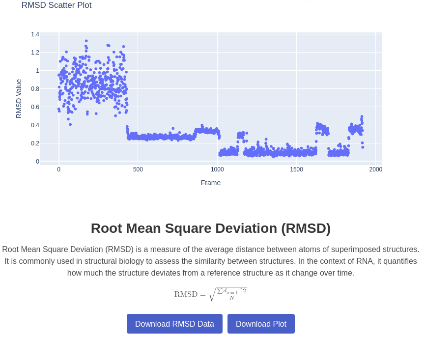
Generates a plot of Root Mean Square Deviation (RMSD) for a given trajectory compared to a native structure. Measures the structural deviation of the trajectory from the native state. RMSD is computed on all the atoms or only heavy atoms, using barnaba function.
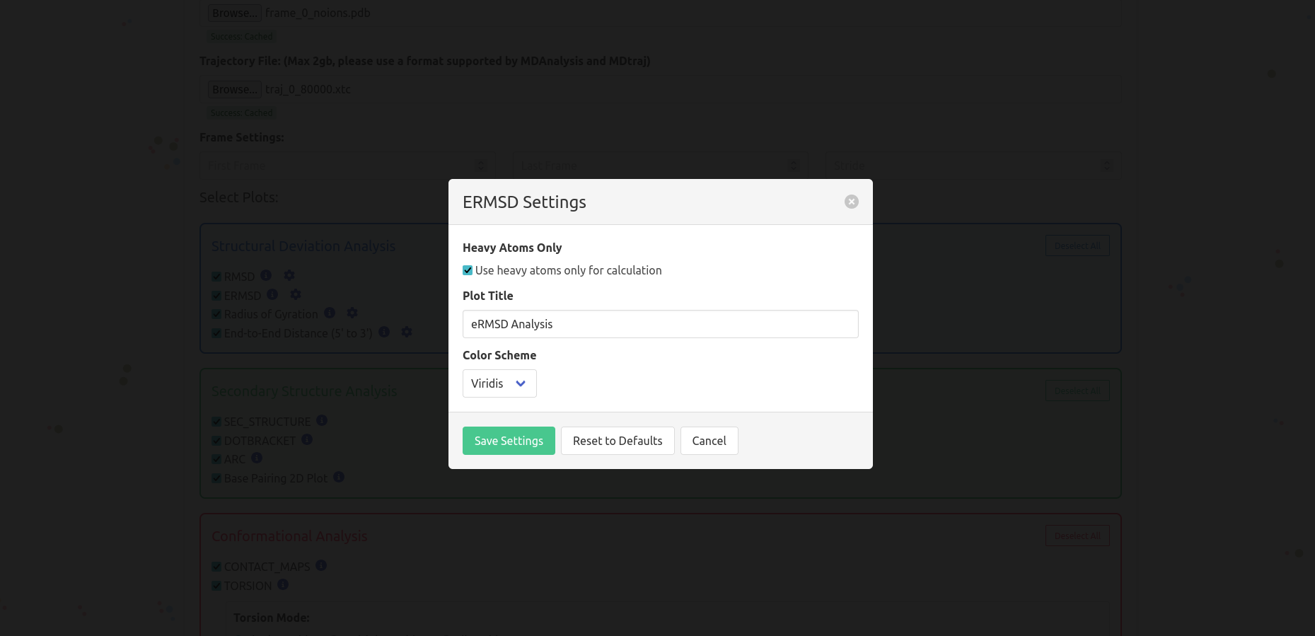
3. ERMSD Plot
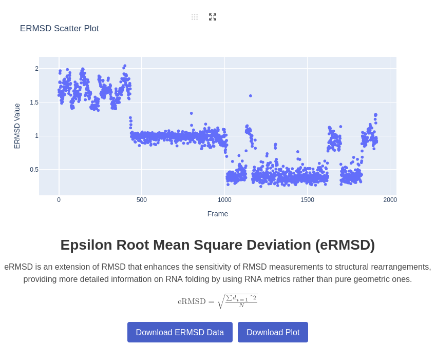
Generates a plot of eRMSD for a given trajectory compared to a native structure. Measures the structural deviation of the trajectory from the native state, taking into account escore, derived from the position of base pairs Bottaro et al., 2014.
5. Secondary Structure Plot
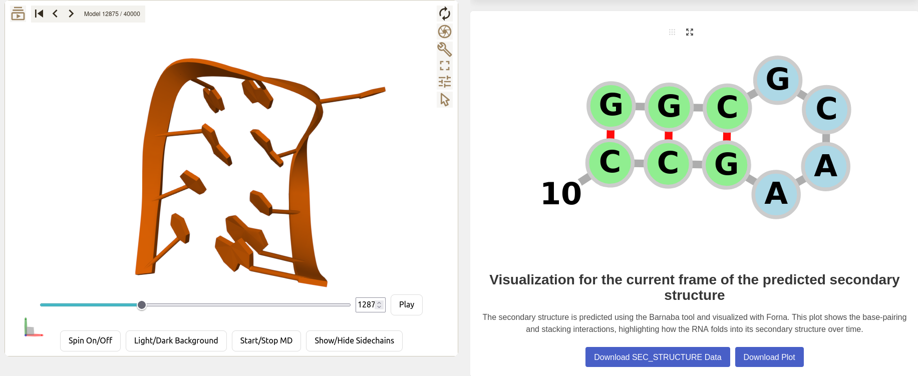
Visualize the secondary structure of the displayed frame, the secondary structure is computed via Barnaba, and the visualisation is done using Forna.
6. Arc Plot
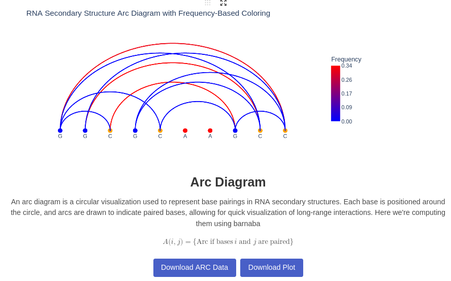
Generates an Arc plot illustrating base pairing interactions within the RNA structure. Each nucleotide is connected to another if a base pair is formed during the trajectory. The color represents the frequency of each contact throughout the trajectory.
8. Dot-Bracket Plot
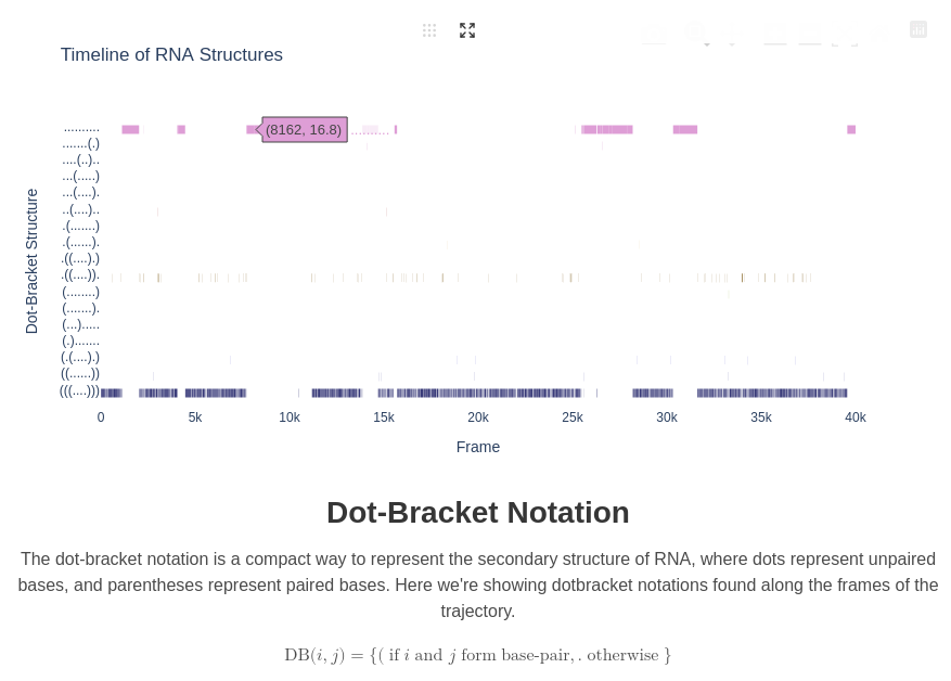
For this plot, we're computing the Dotbracket information (representing in a format of string the secondary structure), and we're ploting along time the position of each dotbracket structure: it gives some insight on how the structure are transitioning from one to another. If they are too much of them (more than 20), only the top 20 by frequency is keeped for clarity purpose.
9. 2D Base Pairing

Visualizes the positions of nucleobases along the trajectory, with color indicating the frequency of their positions. All base position data are aggregated into this plot, meaning precision decreases as the number of nucleotides increases. However, it still provides valuable insights into the forcefield's behavior. Data is obtained using Barnaba and visualized with Plotly.
9. Torsion Angles Plot
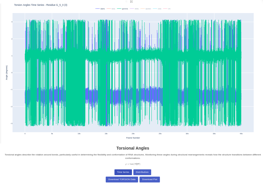
Generates a plot of torsion angles against time or against another torsion angle, for a given trajectory. Visualizes the backbone dihedral angles (alpha, beta, gamma, delta, epsilon, zeta, chi) over the trajectory. You can select specific residues or analyze all residues. Two plots are generated: the first shows the evolution of the angles throughout the trajectory, and the second shows the distribution of values. This analysis provides insights into the local backbone flexibility and conformational preferences.
10. PCA (Principal Component Analysis) Plot
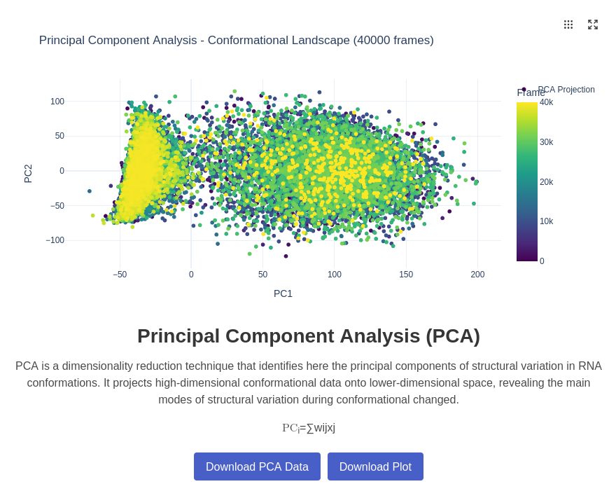
Principal Component Analysis (PCA) reduces the dimensionality of the conformational space by identifying the most significant modes of structural variation in the RNA trajectory. This technique projects the high-dimensional conformational data onto a lower-dimensional space defined by the principal components, revealing the dominant patterns of molecular motion and conformational changes throughout the simulation. The analysis is for the moment only done on 3D coordinates data.
11. UMAP (Uniform Manifold Approximation) Plot
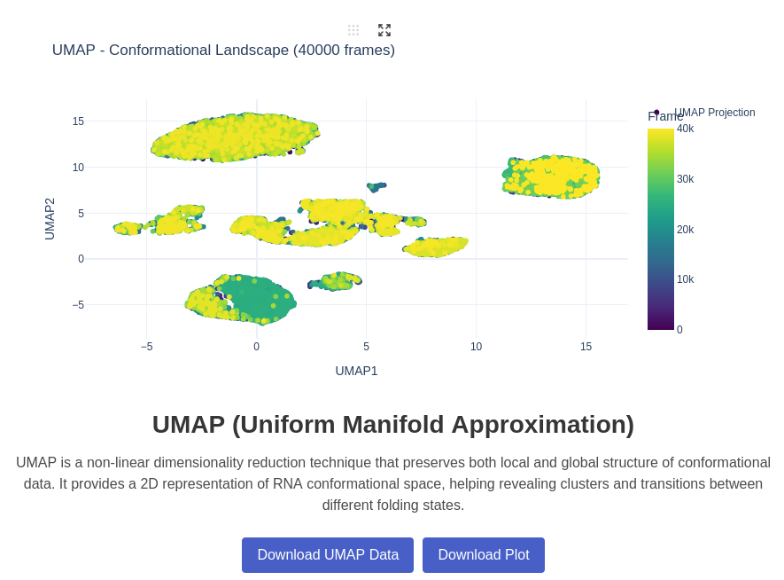
UMAP (Uniform Manifold Approximation and Projection) is a non-linear dimensionality reduction technique that preserves both local and global structure in the data. For RNA conformational analysis, UMAP can reveal complex relationships between different conformational states that might not be apparent with linear methods like PCA, providing insights into the underlying conformational landscape and transition pathways. This analysis is for the moment only done on 3D coordinates data
12. t-SNE (t-Distributed Stochastic Neighbor Embedding) Plot
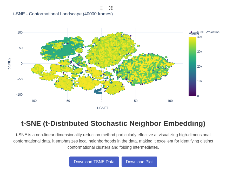
t-SNE (t-Distributed Stochastic Neighbor Embedding) is a machine learning algorithm for non-linear dimensionality reduction that is particularly well-suited for visualizing high-dimensional datasets. In the context of RNA analysis, t-SNE can reveal distinct conformational clusters and help identify rare conformational states or transition intermediates that might be difficult to detect with other methods.
13. Conformational Landscape Plot
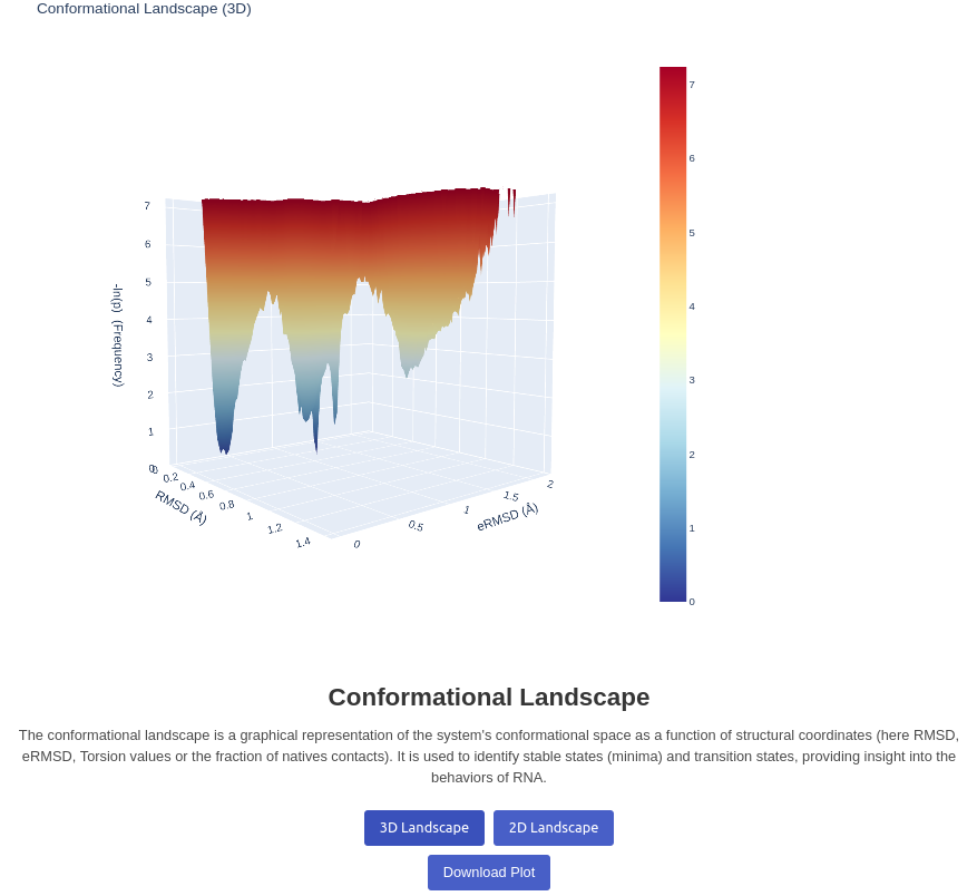
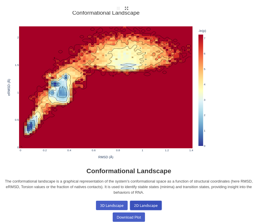
Generates a 2D/3D landscape plot for a given trajectory. Visualizes the energy landscape of the trajectory based on two inputs decided by the user, between RMSD, eRMSD, Torsion and Fraction of native contacts. The depth is calculated by the number of structures found in the same positions, and passed to a log function before display A real calculation using Free Energy is ongoing. Note that you can click on the plots to view to what structure a well correspond to, it will automatically change the frame to the closest structure.
Viewer Settings and Controls
Understanding the molecular viewer interface and its controls
- Frame Slider: Drag to quickly navigate through trajectory frames
- Frame Input Box: Enter a specific frame number for direct navigation
- Play Button: Automatically play through the trajectory animation
- Spin Toggle: Enable/disable continuous rotation of the molecule around its center
- Background Toggle: Switch between light and dark background themes for better contrast
- Sidechain Toggle: Show/hide nucleotide side chains for clearer structural visualization
- Mouse Controls: Left-click drag to rotate, right-click drag to move the structure, middle-click drag to zoom
- Selection Tools: Click on atoms or residues to select and highlight specific parts
- Note that each nucleotide is automatically coloured differently: Adenine in Orange, Uracyl in blue, Guanine red and Cytosine in green.
- Frame Highlighting: Current frame is highlighted in time-series plots with vertical markers
- Interactive Clicking: Click on landscape plots, and on Frame related plots to jump to corresponding frames in the viewer
- Real-time Updates: Contact maps and other frame-dependent plots update automatically when frame changes
- Data Correlation: Hover over plot points to see corresponding structural information
Sources
Bottaro S, Di Palma F, Bussi G. The role of nucleobase interactions in RNA structure and dynamics. Nucleic Acids Res. 2014 Dec 1;42(21):13306-14. doi: 10.1093/nar/gku972. Epub 2014 Oct 29. PMID: 25355509; PMCID: PMC4245972.
Michaud-Agrawal, N., Denning, E.J., Woolf, T.B. and Beckstein, O. (2011), MDAnalysis: A toolkit for the analysis of molecular dynamics simulations. J. Comput. Chem., 32: 2319-2327. https://doi.org/10.1002/jcc.21787
Kerpedjiev P, Hammer S, Hofacker IL. Forna (force-directed RNA): Simple and effective online RNA secondary structure diagrams. Bioinformatics. 2015 Oct 15;31(20):3377-9. doi: 10.1093/bioinformatics/btv372. Epub 2015 Jun 22. PMID: 26099263; PMCID: PMC4595900.
McGibbon RT, Beauchamp KA, Harrigan MP, Klein C, Swails JM, Hernández CX, Schwantes CR, Wang LP, Lane TJ, Pande VS. MDTraj: A Modern Open Library for the Analysis of Molecular Dynamics Trajectories. Biophys J. 2015 Oct 20;109(8):1528-32. doi: 10.1016/j.bpj.2015.08.015. PMID: 26488642; PMCID: PMC4623899.
Plotly: 1. Inc. PT. Collaborative data science [Internet]. Montreal, QC: Plotly Technologies Inc.; 2015.